Let's suppose you have a dataset of numerical values and you would like to make a future estimate based on them. Some real-life applications include:

Product pricing;
Historical production and demand;
Financial assets valuation;
Calibration of a machine through time;
Concentration of chemical reagents and products;
Disease transmission rates;
Water reservoir levels;
Electricity demand;
Fuel consumption.

The least squares fitting is a mathematical tool that generates an equation close to existing measurements. Many types of curves can be used, such as linear, polynomial, exponential, logarithmic, and many others.

Consider the graph below, sales per month. The blue line is the linear approximation and the red line corresponds to the real values.

---
config:
    xyChart:
        width: 540
    themeVariables:
        xyChart:
            backgroundColor: "#00000000"
            plotColorPalette: "#C00, #22F"
---
xychart-beta
    title "Sales per month ($)"
    x-axis "month" [1,2,3,4,5,6,7,8,9,10,11,12]
    y-axis 0 --> 50000
    line [17000, 24000, 16000, 30000, 35000, 26000, 29000, 40000, 44000, 35000, 41000, 47000]
	line [18461.538, 20923.076, 23384.614, 25846.152, 28307.690, 30769.228, 33230.766, 35692.304, 38153.842, 40615.380, 43076.918, 45538.456]
	%% =2461,538 * x + 16000

Theory

Consider f(x) the equation we want to generate and (x_i, y_i) the measurements we have. The best equation is the one where the differences between approximations and measurements are the smallest possible; in other words:

|f(x_i) - y_i| is the distance between approximation and reality;
Σ is the summation.
Σ|f(x_i) - y_i| should be the closest to zero.

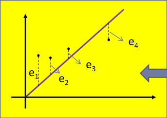
Differences between approximations and measurements.

Let's name SSE the sum of squared errors: SSE = Σ(f(x_i) - y_i)². As our objective is to measure the distance between approximation and reality, we'll simply power square the difference, instead of applying the absolute function; it's easier.

We need to apply an absolute or power square operation for distance measurement because a simple subtraction could result in a negative value, which isn't valid for distances.

The minimum of SSE depends on the type of desired approximation:

Linear: f(x) = ax + b
Exponential: f(x) = a * e^bx
Power law: f(x) = a * x^b
Logarithmic: f(x) = a + b * ln(x)

Substituting f(x) by the functions above in SSE, we'll see that it depends on variables a and b. In the case of linear approximation: SSE(a,b) = Σ(a * x_i + b - y_i)².

The minimum of a function happens on the point where its derivative (slope) equals zero:

---
config:
    xyChart:
        width: 540
    themeVariables:
        xyChart:
            backgroundColor: "#00000000"
            plotColorPalette: "#CC0000, #f59316, #f59316, #f59316"
---
xychart-beta
    title "y = x²"
    x-axis "x" -6 --> 6
    y-axis "y" 0 --> 40
    line [36,25,16,9,4,1,0,1,4,9,16,25,36]
	line [27,21,15,9,3,-3,-9,-15,-21,-27,-33,-39,-45]
    line [0,0,0,0,0,0,0,0,0,0,0]
    line [-45,-39,-33,-27,-21,-15,-9,-3,3,9,15,21,27]

In red: y = x². In orange: the derivatives (slopes) for x = -3, 0 and 3.

SSE will have its minimum point where the partial derivatives relative to a and b are zero, solving the following system:

∂SQE(a,b) / ∂a = 0

∂SQE(a,b) / ∂b = 0

This is the basics for the least squares fitting method. If you are interested and would like to know more, there are links in the end of this page with additional explanations on this topic. Particularly, I recommend this lesson by Stan Brown.

Functional programming

Functional programming is a paradigm that focuses on data transformations: like in a mathematical function, a value x is transformed by f(x). In functional code, transformations are often chained, e.g., f(g(h(x))).

In this article, we will use the F# language, that uses the .NET runtime.

This post explains how to set up your environment and contains tips on the language syntax.

Linear approximation

The equation will be f(x) = a * x + b.

From a set of values (x_i, y_i), a and b are determined by:

The F# code below calculates the linear approximation.

x and y are the input values.
Seq.sumBy sums the results of a function applied over elements of a sequence:
- x = [1, 2, 3]
- x |> Seq.sumBy(fun i -> i * 2) = 12 (2*1 + 2*2 + 2*3 = 12)
Seq.zip makes a sequence of pairs coming from two other sequences:
- x = [1, 2, 3]
- y = [9, 8, 7]
- Seq.zip(x)(y) = [ (1, 9), (2, 8), (3, 7) ].

// s = sum
let s(v: double[]): double =
    v |> Seq.sum

// sm = sum of multiplications
let sm(v1: double[])(v2: double[]): double =
    Seq.zip(v1)(v2)
    |> Seq.sumBy (fun (x, y) -> x * y)

let linearApproximation(x: double[])(y: double[]): (double * double) =
    let n = x.Length |> double
    let sx = s(x)
    let sx2 = sm(x)(x)
    let sy = s(y)
    let sxy = sm(x)(y)
    let d = n*sx2 - sx**2
    let a = (n*sxy - sx*sy)/d
    let b = (sx2*sy - sxy*sx)/d
    (a,b)

Exponential approximation

The equation will be f(x) = A * e^(B * x). e is the natural base, approximately equal to 2.71828.

From a set of values (x_i, y_i), a and b are determined by:

The F# code below calculates the exponential approximation.

ln is the natural logarithm, on base e.
A = e^a.
Seq.zip3 follows the same logic as Seq.zip, but forms a sequence of groups of three, coming from three other sequences.
Important: the values of y need to be all greater than 0, because there is no logarithm of zero or negative numbers.

// s = sum
let s(v: double[]): double =
    v |> Seq.sum

// sm = sum of multiplications
let sm(v1: double[])(v2: double[]): double =
    Seq.zip(v1)(v2)
    |> Seq.sumBy (fun (x, y) -> x * y)

let ln = System.Math.Log

// smm = sum(v1 * v2 * v3)
let smm(v1: double[])(v2: double[])(v3: double[]): double =
    Seq.zip3(v1)(v2)(v3)
    |> Seq.sumBy (fun (a,b,c) -> a * b * c)

// smln = sum(v1 * ln(v2))
let smln(v1: double[])(v2: double[]): double =
    Seq.zip(v1)(v2)
    |> Seq.sumBy (fun (a,b) -> a * ln(b))

// smmln = sum(v1 * v2 * ln(v3))
let smmln(v1: double[])(v2: double[])(v3: double[]): double =
    Seq.zip3(v1)(v2)(v3)
    |> Seq.sumBy (fun (a,b,c) -> a * b * ln(c))

// exponential: y = A * e^(b*x)
let exponentialApproximation(x: double[])(y: double[]): (double * double) =
    let sx2y = smm(x)(x)(y)
    let sylny = smln(y)(y)
    let sxy = sm(x)(y)
    let sxylny = smmln(x)(y)(y)
    let sy = s(y)
    let d = sy*sx2y - sxy**2
    let a = (sx2y*sylny - sxy*sxylny)/d
    let b = (sy*sxylny - sxy*sylny)/d
    let A = System.Math.Exp(a)
    (A, b)

Case study: Silver mining

Pirquitas mine, Jujuy, Argentina.

Let's extract data from the Our World in Data website on world silver mining production, between 1900 and 2023, and let's make the linear and exponential approximations.

CSV data available here.

Results:

f(x) is the mining production in metric tonnes, x is the year.
Linear: f(x) = 162.897 * x - 308090.816
Exponential: f(x) = 0.000000002257 * e^(x * 0.01485166)

---
config:
    xyChart:
        width: 540
    themeVariables:
        xyChart:
            backgroundColor: "#00000000"
            plotColorPalette: "#CC0000, #2222FF, #00CC00"
---
xychart-beta
    title "Silver mining production (metric tonnes)"
    x-axis "Year" 1900 --> 2023
    y-axis 0 --> 30000
    line [ 5400, 5380, 5060, 5220, 5110, 5360, 5130, 5730, 6320, 6600, 6900, 7040, 6980, 7010, 5240, 5730, 5250, 5420, 6140, 5490, 5390, 5330, 6530, 7650, 7450, 7650, 7890, 7900, 8020, 8120, 7740, 6080, 5130, 5340, 5990, 6890, 7920, 8640, 8320, 8300, 8570, 8140, 7780, 6380, 5740, 5040, 3970, 5220, 5440, 5570, 6320, 6210, 6700, 6900, 6670, 7000, 7020, 7190, 7430, 6910, 7320, 7370, 7650, 7780, 7730, 8010, 8300, 8030, 8560, 9200, 9360, 9170, 9380, 9700, 9260, 9430, 9840, 10300, 10700, 10800, 10700, 11200, 11500, 12100, 13100, 13100, 13000, 14000, 15500, 16400, 16600, 15600, 14900, 14100, 14000, 14900, 15100, 16500, 17200, 17600, 18100, 18700, 18800, 18800, 20000, 20800, 20100, 20800, 21300, 22300, 23300, 23300, 24300, 26700, 28000, 27600, 28600, 26500, 25900, 25800, 23500, 25000, 25600, 26000 ]
	line [ 1413.484, 1576.381, 1739.278, 1902.175, 2065.072, 2227.969, 2390.866, 2553.763, 2716.66, 2879.557, 3042.454, 3205.351, 3368.248, 3531.145, 3694.042, 3856.939, 4019.836, 4182.733, 4345.63, 4508.527, 4671.424, 4834.321, 4997.218, 5160.115, 5323.012, 5485.909, 5648.806, 5811.703, 5974.6, 6137.497, 6300.394, 6463.291, 6626.188, 6789.085, 6951.982, 7114.879, 7277.776, 7440.673, 7603.57, 7766.467, 7929.364, 8092.261, 8255.158, 8418.055, 8580.952, 8743.849, 8906.746, 9069.643, 9232.54, 9395.437, 9558.334, 9721.231, 9884.128, 10047.025, 10209.922, 10372.819, 10535.716, 10698.613, 10861.51, 11024.407, 11187.304, 11350.201, 11513.098, 11675.995, 11838.892, 12001.789, 12164.686, 12327.583, 12490.48, 12653.377, 12816.274, 12979.171, 13142.068, 13304.965, 13467.862, 13630.759, 13793.656, 13956.553, 14119.45, 14282.347, 14445.244, 14608.141, 14771.038, 14933.935, 15096.832, 15259.729, 15422.626, 15585.523, 15748.42, 15911.317, 16074.214, 16237.111, 16400.008, 16562.905, 16725.802, 16888.699, 17051.596, 17214.493, 17377.39, 17540.287, 17703.184, 17866.081, 18028.978, 18191.875, 18354.772, 18517.669, 18680.566, 18843.463, 19006.36, 19169.257, 19332.154, 19495.051, 19657.948, 19820.845, 19983.742, 20146.639, 20309.536, 20472.433, 20635.33, 20798.227, 20961.124, 21124.021, 21286.918, 21449.815 ]
	line [ 4059.94, 4120.69, 4182.34, 4244.92, 4308.44, 4372.90, 4438.33, 4504.74, 4572.14, 4640.55, 4709.99, 4780.46, 4851.99, 4924.58, 4998.27, 5073.06, 5148.96, 5226.00, 5304.20, 5383.56, 5464.11, 5545.87, 5628.85, 5713.07, 5798.55, 5885.31, 5973.37, 6062.75, 6153.46, 6245.53, 6338.98, 6433.83, 6530.10, 6627.80, 6726.97, 6827.62, 6929.78, 7033.47, 7138.71, 7245.52, 7353.93, 7463.96, 7575.64, 7689.00, 7804.04, 7920.81, 8039.32, 8159.61, 8281.70, 8405.62, 8531.39, 8659.04, 8788.60, 8920.10, 9053.56, 9189.03, 9326.52, 9466.07, 9607.70, 9751.46, 9897.36, 10045.45, 10195.76, 10348.31, 10503.15, 10660.30, 10819.81, 10981.70, 11146.01, 11312.78, 11482.05, 11653.85, 11828.22, 12005.20, 12184.83, 12367.15, 12552.19, 12740.00, 12930.62, 13124.10, 13320.47, 13519.78, 13722.07, 13927.38, 14135.77, 14347.28, 14561.95, 14779.83, 15000.97, 15225.43, 15453.24, 15684.46, 15919.13, 16157.32, 16399.08, 16644.45, 16893.49, 17146.26, 17402.81, 17663.20, 17927.49, 18195.73, 18467.98, 18744.31, 19024.77, 19309.43, 19598.34, 19891.58, 20189.21, 20491.29, 20797.89, 21109.08, 21424.93, 21745.50, 22070.86, 22401.10, 22736.28, 23076.47, 23421.75, 23772.20, 24127.89, 24488.90, 24855.32, 25227.21 ]
	%% linear: 162,897 * year - 308090,816
	%% exponential: =(0,000000002257)*e^(year*0,01485166)

Red line: year production; blue line: linear approximation; green line: exponential approximation.

Sources and interesting reads

Least squares fitting with functional programming